在整个大语言模型学习之路中,对 Attention 机制的理解大概是最为让我困惑的部分,最终经过层层解构、加上重新把“线性代数”温习了一遍之后,最终,总算某种程度的理解了 Attention 机制的设计。相信对于所有NLP专业的人,这部分都是不太容易理解的。
1. 概述 要想讲清楚,大概也是非常不容易的,这里就做一个尝试吧。这里的重点是讲清楚 Attention Score (简称Attention)的计算。介绍的顺序是“两个词语的相似度”、“Similarity Score Matrix”、“Attention Score Matrix”。
1.1 要构建的是直觉,而不是“推理” 为什么 Attention 理解起来很难呢?我想其中有一个原因大概是这个“机制”本身并不是某种“公式推导”出来的,而是通过一篇篇论文与实践,被证明非常有效的一个机制,所以,这个机制本身的所具备的“可解释性”其实也是有限的。这大概也是,无论你在互联网上如何搜索,也没有谁可以比较简单的把这个机制说清楚的原因。但,理解这个机制构建的直觉,对于理解整个 Transformer ,以及整个当代大语言模型技术基础都是至关重要的。
2. 预处理 在“大语言模型的输入:tokenize ”中详细介绍了“提示词”进入大模型处理之前,如何将提示词换行成大模型可以处理的“词向量”或者说“token embedding”。
大语言模型在开始“Attention”计算之前,还会对“token embedding”进行一些预处理,这些预处理包括了“融入”位置向量、对向量进行“归一化”处理(将各个向量都转化为均值为0、方差为1的向量,长度要统一变成1吗?)。
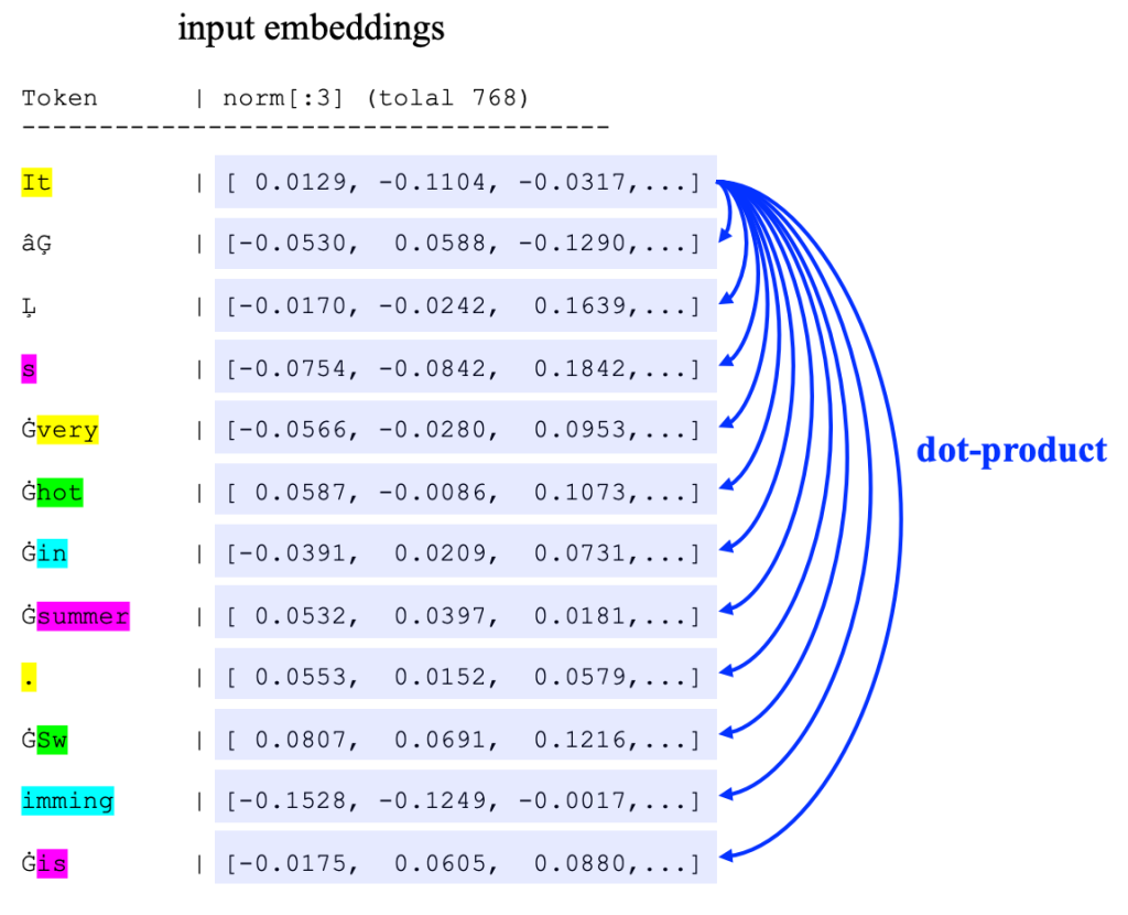
例如,在这里的例子中,提示词 “It’s very hot in summer. Swimming is ”,先转换为embedding,然后加上位置编码(positional encoder)、再进行正规化,最后变换为如下的向量 “ X ” :
|-------------------------------------------------------------------------------------------------------------------------------------------Token | wte[:3] (word token embedding) | wpe[:3](word positional e..) | wte [:3] + wpe [:3] | X[:3] (Norm) |
这里的 “X” 是一个由12个 “token embedding”组成的矩阵,“形状”是 12 x 768 。在数学符号上,有:
--------------------------------------- ------------------------------------------ -------------x_1 = [ 0.0129, -0.1104, -0.0317,...] | |It |x_2 = [-0.0530, 0.0588, -0.1290,...] | |âĢ |x_3 = [-0.0170, -0.0242, 0.1639,...] | |Ļ |x_4 = [-0.0754, -0.0842, 0.1842,...] | |s |x_5 = [-0.0566, -0.0280, 0.0953,...] | |Ġvery |X = [ 0.0587, -0.0086, 0.1073,...] | | x_6 = [ 0.0587, -0.0086, 0.1073,...] | |Ġhot |x_7 = [-0.0391, 0.0209, 0.0731,...] | |Ġin |x_8 = [ 0.0532, 0.0397, 0.0181,...] | |Ġsummer |x_9 = [ 0.0553, 0.0152, 0.0579,...] | |. |x_10 = [ 0.0807, 0.0691, 0.1216,...] | |ĠSw |x_11 = [-0.1528, -0.1249, -0.0017,...] | |imming |x_12 = [-0.0175, 0.0605, 0.0880,...] | |Ġis |
3. Similarity Score Matrix 在正式介绍 Attention 之前,为了能够比较好的理解“为什么”是这样,这里先引入了“Similarity”的概念,最终在该概念上,新增权重矩阵,就是最终的 Attention :
$$ \text{Similarity} = \text{softmax}(\frac{XX^{T}}{\sqrt{d}})X $$
这里删除了参数矩阵:\(W^Q \quad W^K \quad W^V \)
$$ \text{Attention} = \text{softmax}(\frac{QK^{T}}{\sqrt{d}})V $$
其中, \(Q = XW^Q \quad K = XW^K \quad V = XW^V \)
3.1 两个“词语”的相似度 在向量为单位长度的时候,通常可以直接使用“内积”作为两个向量的相似度度量。例如,考虑词语 “hot” 与 “summer” 的相似度,则可以“简化”的处理这两个词(Token)的向量的“内积”。
在前面的文章“大语言模型的输入:tokenize ”中,较为详细的介绍了大语言模型如何把一个句子转换成一个的 Token,然后再转换为一个个“向量”。那么,我们通常会通过两个向量的余弦相似度来描述其相似度,如果向量的“长度”(\(L_2 \) 范数)是单位长度,那么也通常会直接使用“内积”描述两个向量的相似度:
$$
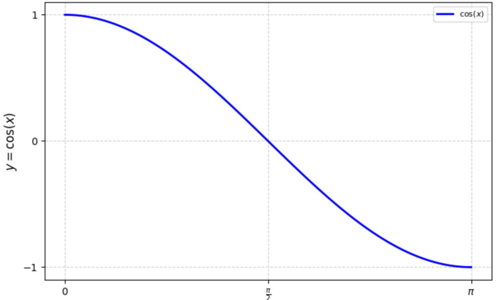
\(f(x) = \cos(x) \) 的图像如右图,故:
夹角为 0 时,最为相似,这时候 \(\cos(x) = 1 \)
夹角 \(\pi \) 时,最“不”相似,这时候 \(\cos(x) = 0 \)
例如,
3.2 “Similarity Score Matrix” 因为两个向量的“内积”某种程度可以表示为相似度。那么,对于句子中的某个 token 来说,与其他所有向量各自计算“内积”,就可以获得一个与其他所有向量“相似程度”的数组,再对这个数组进行 softmax 计算就可以获得一个该 token 与其他所有向量“相似程度”的归一化数组。这个归一化的数据,就可以理解为这里的“Similarity Score Matrix”。
这里依旧以“大语言模型的输入:tokenize ”示例中的句子为演示示例。
更为具体的,可以参考右图。这里考虑 Token “It” 与其他所有词语的相似度。即计算 Token “It” 的 Embedding 向量,与其他所有向量的“内积”。
更进一步,如果计算两两词语之间的相似度,并进行归一化(softmax ),则有如下的Similarity Matrix:
[0.6975, 0.0347, 0.0236, 0.0298, 0.0386, 0.0282, 0.0272, 0.0270, 0.0216, 0.0244, 0.0219, 0.0254]
在这个示例中,则会有上述 12×12 的矩阵。该矩阵反应了“词”与“词”之间的相似度。如果,我们把每一行再进行一个“归一化”(注右图已经经过了归一化),那么每一行,就反应了一个词语与其他所有词语相似程度的一个度量。
例如,右图中 it 可能与 very 最为相似(除了自身)。
4. Self-Attention 4.1 对比 注意到最终的 “Attention” 计算公式和上述的“Similarity Score Matrix”的差别就是参数矩阵W:
$$ \text{Similarity Score} = \text{softmax}(\frac{XX^{T}}{\sqrt{d}})X $$
这里没有参数矩阵:\(W^Q \quad W^K \quad W^V \)
$$ \text{Attention} = \text{softmax}(\frac{QK^{T}}{\sqrt{d}})V $$
其中, \(Q = XW^Q \quad K = XW^K \quad V = XW^V \)
4.2 为什么需要参数矩阵 W 那么,为什么需要 \(W^Q \,, W^K \,, W^V \) 呢?这三个参数矩阵乘法,意味着什么呢?要说清楚、要理解这个点并不容易,也没有什么简单的描述可以说清楚的,这也大概是为什么,对于非 NLP 专业的人,要想真正理解 Transformer 或 Attention 是比较困难的。
你可能会看到过一种比较普遍的、简化版本,大概是说 \(W^Q \) 是一个 Query 矩阵,表示要查询什么;\(W^K \) 是一个 Key 矩阵,表示一个词有什么。这个说法似乎并不能增加对上述公式的理解。
那么,一个向量乘以一个矩阵时,这个“矩阵”意味着什么?是的,就是“线性变换”。
4.3 线性变换 Linear Transformations 一般来说,\(W^Q \,, W^K \,, W^V \) 是一个 \(d \times d \) 的矩阵[1] 。对于的 Token Embedding (上述的矩阵 X )所在的向量空间,那么 \(W^Q \,, W^K \,, W^V \) 就是该向量空间的三个“线性变换”。
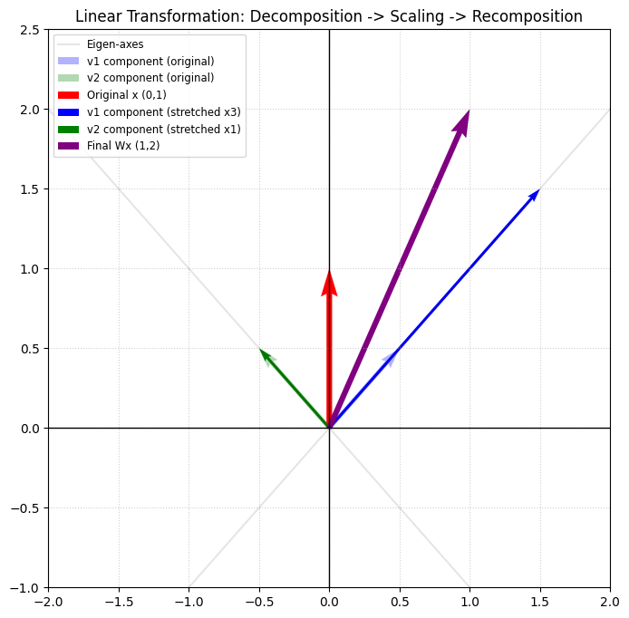
那么线性变换对于向量空间的作用是什么呢?这里我们以“奇异值分解”的角度来理解这个问题[2] ,即对向量进行拉伸/压缩、旋转、镜像变换。\(W^Q \,, W^K \,, W^V \) 则会分别对向量空间的向量(即Token Embedding)做类似的变换。变换的结果即为:
$$ Q = XW^Q \quad \quad K = XW^K \quad \quad V = XW^V $$
那么,如果参数矩阵“设计”合理,“Token”与“Token”之间就可以建立“期望”的 Attention 关系,例如:“代词”(it),总是更多的关注于“名词”;“名词”更多的关注与附近的“形容词”;再比如,“动词”更多关注前后的“名词”等。除了词性,线性变换关注的“维度”可能有很多,例如“位置”、“情感”、“动物”、“植物”、“积极/消极”等。关于如何理解 token embedding 的各个“维度”含义可以参考:Word Embedding 的可解释性探索 。
当然,这三个参数矩阵都不是“设计”出来的,而是“训练”出来的。所以,要想寻找上述如此清晰的“可解释性”并不容易。2019年的论文《What Does BERT Look At? An Analysis of BERT’s Attention 》较为系统的讨论了这个问题,感兴趣的可以去看看。
关于线性变换如何作用在向量空间上,可以参考:线性代数、奇异值分解–深度学习的数学基础 。
所以,\( \frac{QK^T}{\sqrt{d}} = \frac{XW^Q (XW^K)^T}{\sqrt{d}} \) 则可以系统的表示,每个“Token”对于其他“Token”的关注程度(即pay attention的程度)。可以注意到:
增加了参数矩阵\(W^Q \,, W^K \,, W^V \)后,前面的“相似性”矩阵,就变为“注意力”矩阵
“Token” 之间的关注程度不是对称的。例如 Token A 可能很关注 B;但是 B 可能并不关注 A
这里的 \(\sqrt{d} \) 根据论文描述,可以提升计算性能;
如果,你恰好理解了上面所有的描述,大概会有点失望的。就只能到这儿吗?似乎就只能到这里了。如果,你有更深刻的理解,欢迎留言讨论。
接下里,我们来看看 “Attention Score Matrix” 的计算。
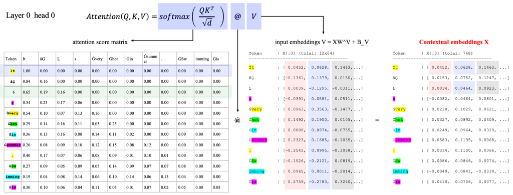
4.4 Attention Score Matrix 使用上述的 “Similarity Score Matrix” 的计算方式,可以计算类似的 “Attention Score Matrix”,之后再对该矩阵进行 softmax 计算就可以获得每个词语对于其他所有词语的 Attention Score,或者叫“关注程度”。有了这个关注程度,再乘以 V 矩阵,原来的 Token Embedding 就变换为一个新的带有上下文的含义的 Token Eembedding 了,即 Context Embedding[3] 。
类似的,我们有右图的 Attention Score Matrix 计算。
该矩阵反应了两个 Token 之间的 Attention 关系。该关系,通过对经过线性变换的 Token Embedding ,再进行内积计算获得。
Attention Score Matrix (12 x 12)
4.5 Masked Attention Score Matrix 上述计算,是一个典型的 Self Attention 计算过程,BERT 模型就使用类似的计算,但 GPT 模型(或者叫 Decoder 模型)还有一些不同。GPT 模型中为了训练出更好的从现有 Token 中生成新 Token 的模型,将上述的 Self Attention 更改成了 Masked Self Attention ,即将 Attention Score Matrix 的右上角部分全部置为 -inf (即负无穷),后续经过 softmax 之后这些值都会变成零,即,在该类模型下,一个词语对于其后面的词的关注度为 0 。
在 Decoder 模型设计中,为了生成更准确的下一个 Token 所以在训练和推理中,仅会计算Token 对之前的 Token 的 Attention ,所以上述的矩阵的右上角部分就会被遮盖,即就是右侧的 “Masked Attention Score Matrix”。
Masked Attention Score Matrix (12 x 12)
通常为了快速计算对于上述的计算值会除以 \(\sqrt{d} \) ,可以提升计算的效率。
4.6 归一化(softmax) Attention Score 对于上述矩阵的每一行都进行一个 softmax 计算,就可以获得一个归一化的按照百分比分配的Attention Score。
经过归一化之后,每个词语对于其他词语的 Attention 程度都可以使用百分比表达处理。例如,“summer”对于“It”的关注程度最高,为26%;其次是关注“hot”,为15%。可以看到这一组线性变换(\(W^Q\,W^K \))对于第一个位置表达特别的关注。
The Attention Score Matrix (12 x 12)
4.7 Contextual Embeddings 最后,再按照上述的 Attention Matrix 的比例,将各个 Token Embedding 进行一个“加权平均计算”。
例如,上述的加权计算时,“summer” 则会融入 26% 的“It”,15%的“hot”… ,最后生成新的 “summer” 的表达,这个表达也可以某种程度理解为 “Contextual Embeddings”。需要注意的是,这里在计算加权平均,也不是直接使用原始的 Token Embedding ,也是一个经过了线性变换的Embedding,该线性变换矩阵也是经过训练而来的,即矩阵 \(W^V \)。
例如,上述的加权计算时,“summer” 则会融入 26% 的“It”,15%的“hot”… ,最后生成新的 “summer” 的表达,这个表达也可以某种程度理解为 “Contextual Embeddings”。
需要注意的是,这里在计算加权平均,也不是直接使用原始的 Token Embedding ,也是一个经过了线性变换的Embedding,该线性变换矩阵也是经过训练而来的,即矩阵 \(W^V \)。
Token | Contextual Embeddings(12 x 768)
5 计算示意图 如下的示意图,一定的可视化的表达了,一个 Token 如何经过上述的矩阵运算,如何了其他 Token 的内容。
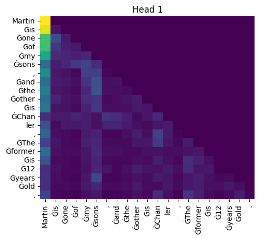
6. 注意力矩阵的观察 那么,我们给定于如下的提示词输入:“Martin’s one of my sons, and the other is Chanler.”。看看在 GPT 模型中,各个Token之间的 Attention 情况:
这句话总计有21个token,所以这是一个21×21的矩阵
这里是“masked self-attention”,所以矩阵的右上半区都是 “0” 。
在GPT2中,一共12层,每层12个“头”,所以一共有“144”个类似的矩阵
\(W^Q \,, W^K \,, W^V \) 的维度都是768×64,所以粗略的估计这部分的参数量就超过2000万,具体的:
768*64*3*144 = 21,233,664
7. Multi-Head Attention 7.1 Scaled Dot-Product Attention 以前面小结“预处理”中的 X 为例,Attention Score Matrix 就有如下的计算公式:
$$
最终的 Attention 计算如下:
$$
7.2 Multi-Head Attention 上述的“Attention”在论文“Attention Is All You Need”称为“Scaled Dot-Product Attention”。更进一步的在论文中提出了“Multi-Head Attention”(经常被缩写为“MHA”)。对应的公式如下(来自原始论文):
$$
更完整的解释,可以参考原始论文。这里依旧以前文的示例来说明什么是MHA。
在本文第4章“Self-Attention”中,较为详细的介绍了相关的计算(即模型的推理过程)。在示例中,一共有12个“Token”,在进入 Attention 计算时经过位置编码、正则化后,12个“Token”向量组成矩阵“X”,这里的“X”的 shape 为 12 x 768,通常使用符号 \(l \times d \) 或者 \(l \times d_{model} \) 表示。最终输出的 Contextual Embedding 也是 \(l \times d_{model} \) 的一组表示12个 Token 向量,这是每个向量相比最初的输入向量,则融合上下文中其他词语的含义。在一个多层的模型中,这组向量则可以作为下一层的输入。
在“Multi-Head Attention”其输入、输出与“Self-Attention”一样,都是 \(l \times d_{model} \) 。但是,对于最终输出的 \(l \times d_{model} \) 的向量/矩阵,在 MHA 中则分为多个 HEAD 各自计算其中的一部分,例如,一共有 \(d_{model} \) 列,那么则分别有 \(h \) 个HEAD,每个 HEAD 输出其中的 \(\frac{d_{model}}{h} \) 列。在上述示例中,供有12个HEAD,即 \(h=12 \),模型维度为768,即\(d_{model} = 768 \),所以每个HEAD,最终输出 \(64 = \frac{d_model}{h} = \frac{768}{12} \) 列。即:
$$
然后由12个 Head 共同组成(concat)要输出的 Contextual Embedding,并对此输出做了一个线性变换\(W^O \)。即:
$$
7.3 Self Attention vs MHA
Self Attention
Multi Head Attention
7.4 Multi-Head Attention 小结
“Multi-Head Attention” 与 经典“Attention” 有着类似的效果,但是有着更好的表现性能
“Multi-Head Attention” 与 经典“Attention” 有相同的输入,相同的输出
8. Attention 数学计算示意图 如下的图片,半可视化的展示了在GTP2中,某一个HEAD中Attention的计算。
9. 全流程数学计算 完整的计算,就是一个“forward propagation”或者叫“inference”的过程,这里依旧以上述的提示词“It’s very hot in summer. Swimming is”,并观察该提示词在 GPT2 模型中的第一个Layer、第一个Head中的计算。完成的代码可以参考:Attention-Please.ipynb
9.1 Token Embedding 和 Positional Embedding
Token Embedding
+
Positional Embedding
|------------ ----------------------------------- ------------------------------- ------------------------------
9.2 Normalize
即,将每一个token的embedding 进行正规化,将其均值变为0,方差变为1
Token | X norm[:3] (12 x 768)
9.3 Attention 层的参数矩阵
W^Q [:3] shape (768 x 64) W^K [:3] shape (768 x 64) W^V [:3] shape (768 x 64)
9.4 矩阵 Q K V的计算
\(Q = XW^Q \)
\(K = XW^K \)
\(V = XW^V \)
Q [:3] shape (12 x 64) K [:3] shape (12 x 64) V [:3] shape (12 x 64)
9.5 计算 Attention Score
\(\text{Attention Score} \)
\(= \frac{QK^T}{\sqrt{d}} \)
|---------------------------------------------------------------------------------------------|
9.6 计算 Masked Attention Score
\(\text{Masked Attention Score} \)
\(= \frac{QK^T}{\sqrt{d}} + \text{mask} \)
|---------------------------------------------------------------------------------------------|
9.7 计算 Softmax Masked Attention Score
\(\text{Softmax Masked Attention Score} \)
\(= \text{softmax}(\frac{QK^T}{\sqrt{d}} + \text{mask}) \)
|-------------------------------------------------------------------------------------|
9.8 计算 Contextual Embeddings
\(\text{Contextual Embeddings} \)
\(= \text{softmax}(\frac{QK^T}{\sqrt{d}} + \text{mask})V \)
Token | Contextual Embedding (12 x 768)
10. 其他 上述流程详述了 LLM 模型中 Attention 计算的核心部分。也有一些细节是省略了的,例如,
在GPT2中,“线性变换”是有一个“截距”(Bias)的,所以也可以称为一个“仿射变换”,即在一个线性变换基础上,再进行一次平移;
在GTP2中,Attention计算都是多层、多头的,本文主要以Layer 0 / Head 0 为例进行介绍;
在生成最终的“Contextual Embeddings”之前,通常还需要一个MLP层(全连接的前馈神经网络)等,本文为了连贯性,忽略了该部分。
总结一下,本文需要的前置知识包括:矩阵基本运算、矩阵与线性变换、SVD 分解/特征值特征向量、神经网络基础、深度学习基础等。
注
[1] 多头注意情况可能是 \(d \times \frac{d}{h} \)
[2] 对于满秩方阵也可以使用“特征值/特征向量”的方式去理解
[3] 在 GPT 2 中,一个 Attention 层的计算,会分为“多头”去计算;并在计算后,还会再经过一个 MLP 层