在开始之前,也没想到99行代码就够了,原以为里面有个“梯度下降”,代码行数应该是数百级别吧,实际完成后,发现加上注释(约35%)才99行。
目录
“极简”神经网络的结构
先来看“极简”有多简:
- 一个输入层、一个输出层,中间没有隐藏层
- 输入层的样本数据就一个特性(feature),总计6个样本
- 这是二分类问题,所以输出层就一个输出值
   x ->   w*x + b   ->   logistic function  -> output
        ----------------------------------
             |                    |
             V                    V
         one neuron     activation function
在后续的实现中,我们构造了六个样本用于该神经网络的训练。
鉴于这个“极简”神经网络,没有任何隐藏层,所以,这也是一个典型的“logistic regression”问题。
前置知识
你需要了解如下的前置知识,以很好的理解该神经网络的实现与训练:
- 了解神经网络的基础:浅层神经网络
- 了解 梯度下降算法,了解基本最优化算法概念,了解链式法则
- 了解 logistic function 的基本特性
- 了解 Python 和 NumPy 的基本使用
问题描述与符号约定
用于训练的样本数据有\( (x,\hat{y}) \): \( (1,0)、(2,0)、(3,0)、(4,0)、(5,1)、(6,1) \)。
一个具体的样本,在下面的公式中通常使用 \( (x^{(j)}, y^{(j)}) \)表示, 其中,\( j = 1…m \)。
\( \hat{y} \)则表示根据参数计算出的预测值,更为具体的 \( \hat{y}^{(j)} \)表示 \(x = x^{(j)} \)时的预测值。
构建目标函数
从样本数据可以看到,这是一个二分类问题,可以使用logistic function作为输出层的激活函数,如果输出值大于0.5,则预测为1,否则预测为0。
对于任何一个样本,就可以如下函数作为logistic function的损失函数\( L \):
$$
L(y,\hat{y}) = – (yln(\hat{y}) + (1-y)ln(1-\hat{y}))
$$
所以,全局的目标函数就是:
$$
\begin{aligned}
J(w,b) & = \frac{1}{m} \sum\limits_{j=0}^{m} L(y^{(j)},\hat{y}^{(j)}) \\
& = \frac{1}{m} \sum\limits_{j=0}^{m} – (y^{(j)}ln(\hat{y}^{(j)}) + (1-y^{(j)})ln(1-\hat{y}^{(j)}))
\end{aligned}
$$
其中 \( m \)表示总样本数量,这里取值是6。在这个极简的神经网络中 \( \hat{y} \)有如下计算表达式:
$$
\hat{y} = \frac{1}{1+e^{-(wx+b)}}
$$
最终,该神经网络的参数求解(也就是“训练”)过程,就是求解如下的极值问题:
$$
(w,b) = \min_{w, b} J(w, b) = \min_{w,b} \frac{1}{m} \sum\limits_{j=0}^{m} L(y^{(j)},\hat{y}^{(j)})
$$
目标函数计算的具体代码如下:
def cost_function(w_p,b_p,x_p,y_p):
    c = 0
    for i in range(m):
        y = function_f(x_p[i],w_p,b_p)
        c += -y_p[i]*math.log(y) - (1-y_p[i])*math.log(1-y)
    return c
梯度计算
前面介绍了很多梯度的内容,这里不再详述。在这个具体的问题中,需要求解的梯度为:
$$
(\frac{\partial J}{\partial w},\frac{\partial J}{\partial b})
$$
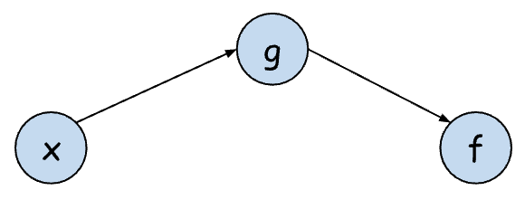
在这里,简单展示该梯度的计算,主要需要使用的是链式法则和基本的求导/微分运算。
首先,为了便于计算,这里记:
$$
\begin{aligned}
\hat{y} & = \frac{1}{1+e^{-z}} \\
z & = w*x + b
\end{aligned}
$$
所以,根据链式法则容易有:
$$
\frac{\partial L}{\partial w} = \frac{\partial L}{\partial \hat{y}} * \frac{\partial \hat{y}}{\partial z} * \frac{\partial z}{\partial w} \\
\frac{\partial L}{\partial b} = \frac{\partial L}{\partial \hat{y}} * \frac{\partial \hat{y}}{\partial z} * \frac{\partial z}{\partial b}
$$
这其中,\( \frac{\partial L}{\partial \hat{y}} \) 和 \( \frac{\partial \hat{y}}{\partial z} \)略有一些计算量,\( \frac{\partial z}{\partial w} \) 和\( \frac{\partial z}{\partial b} \)比较简单,具体的:
$$
\begin{aligned}
\frac{\partial L}{\partial \hat{y}} * \frac{\partial \hat{y}}{\partial z} & = \hat{y} – y \\
\frac{\partial z}{\partial w} & = x \\
\frac{\partial z}{\partial b} & = 1
\end{aligned}
$$
所以,最终的梯度计算公式如下:
$$
\begin{aligned}
\frac{\partial J}{\partial w} & = \frac{1}{m} \sum\limits_{j=1}^{m} (\hat{y}^{(j)} – y^{(j)})*x^{(j)} \\
\frac{\partial J}{\partial b} & = \frac{1}{m} \sum\limits_{j=1}^{m} (\hat{y}^{(j)} – y^{(j)})
\end{aligned}
$$
在实际的计算中,先通过正向传播(Forward Propagation)计算出\( \hat{y}^{(j)} \),然后在计算出梯度。此外,可以使用NumPy的ndarray简化表达,同时增加计算的并行性。这里为便于理解,全部都使用标量计算,在文章的最后也提供了NumPy的对应实现。
正向传播计算如下:
# function_f:
# x   : scalar
# w   : scalar
# b   : scalar
def function_f(x,w,b):
    return 1/(1+math.exp(-(x*w+b)))
梯度(反向传播)计算如下:
# Gradient caculate
# x_p: x_train
# y_p: y_train
# w_p: current w
# b_p: current b
def gradient_caculate(x_p,y_p,w_p,b_p):
    gradient_w,gradient_b = (0.,0.)
    for i in range(m):
        gradient_w += x_p[i]*(function_f(x_p[i],w_p,b_p)-y_p[i])
        gradient_b += function_f(x_p[i],w_p,b_p)-y_p[i]
    return gradient_w,gradient_b
梯度下降迭代
这里设置迭代次数为50000次,学习率设置为0.01,当迭代目标函数变化值小于0.000001时也停止迭代(这并不是必须的)。具体的:
iteration_count = 50000
learning_rate = 0.01
cost_reduce_threshold = 0.000001
于是又如下梯度下降迭代过程的代码:
cost_last = 0
for i in range(iteration_count):
    grad_w,grad_b = gradient_caculate(x_train,y_train,w,b)
    w = w - learning_rate*grad_w
    b = b - learning_rate*grad_b
    cost_current = cost_function(w,b,x_train,y_train)
    if i >= iteration_count/2 and cost_last - cost_current<= cost_reduce_threshold:
        print("iteration: {:5d},cost_current:{:f},cost_last:{:f},cost reduce:{:f}".format( i+1,cost_current,cost_last,cost_last-cost_current))
        break
    if (i+1)%(iteration_count/10) == 0:
        print("iteration: {:5d},cost_current:{:f},cost_last:{:f},cost reduce:{:f}".format( i+1,cost_current,cost_last,cost_last-cost_current))
    cost_last = cost_current
预测
完成训练后,则可以对输入值进行预测。代码如下:
print("after the training, parameter w = {:f} and b = {:f}".format(w,b))

for i in range(m):
    y = function_f(x_train[i],w,b)
    p  = 0
    if y>= 0.5: p  = 1
    print("sample: x[{:d}]:{:d},y[{:d}]:{:d}; the prediction is {:d} with probability:{:4f}".format(i,x_train[i],i,y_train[i],p,y))
上述代码会产生如下的输出:
after the training, parameter w = 5.056985 and b = -22.644516
sample: x[0]:0,y[0]:0; the prediction is 0 with probability:0.000000
sample: x[1]:1,y[1]:0; the prediction is 0 with probability:0.000000
sample: x[2]:2,y[2]:0; the prediction is 0 with probability:0.000004
sample: x[3]:3,y[3]:0; the prediction is 0 with probability:0.000568
sample: x[4]:4,y[4]:0; the prediction is 0 with probability:0.081917
sample: x[5]:5,y[5]:1; the prediction is 1 with probability:0.933417
可以看到,在完成训练后的这个极简神经网络能够较为准确的预测样本中的数据。
完整的代码
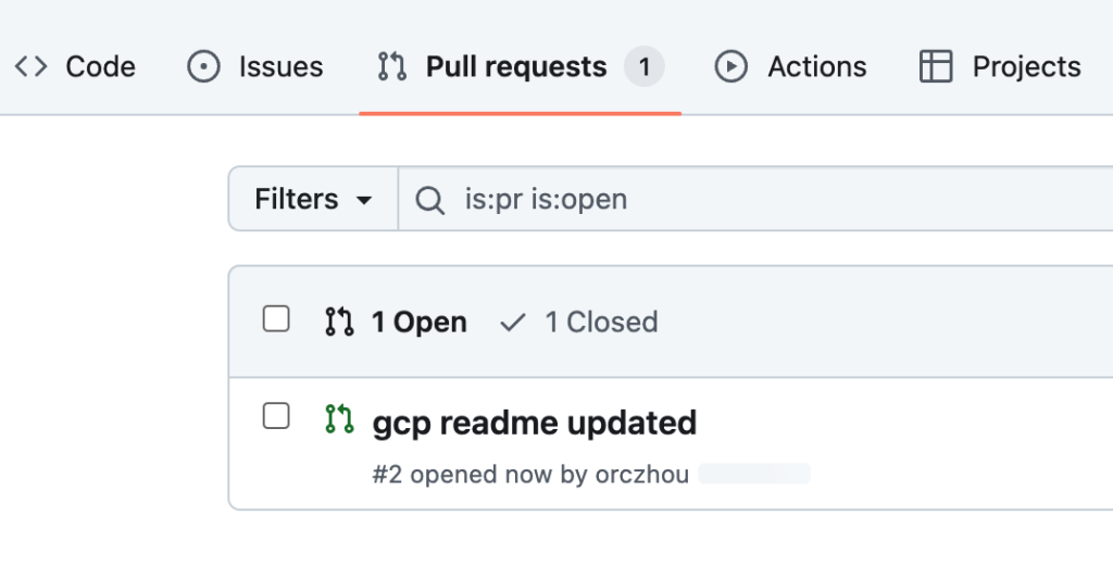
完成在的代码可以在 GitHub 上查看:https://github.com/orczhou/ssnn/ 。包括了三个段程序:
- ssnn_ant.py : 最为基础的上述神经网络的实现
- ssnn_ant_np.py : 使用numpy对上述实现进行向量化
- ssnn_ant_tf.py : 使用 TensorFlow 框架实现上述程序
这里也简单列出相关程序如下(最新代码可以参考上述 GitHub 仓库):
ssnn_ant.py
"""
super simple neural networks
  * only one neuron in only the one hidden layer
  * input x is scalar (one-dimension)
  * using logistic function as the activation function

input layer:
    x: scalar
parameters:
    w: scalar
    b: scalar
output:
    y \in [0,1] or  p \in {0,1}
structure:

   x ->   w*x + b   ->   logistic function  -> output
        -----------      -----------------
             |                    |
             V                    V
         one neuron     activation function

about it:
    it's a simple project for human learning how machine learning
    by orczhou.com
"""
import numpy as np
import math

# function_f:
# x   : scalar
# w   : scalar
# b   : scalar
def function_f(x,w,b):
    return 1/(1+math.exp(-(x*w+b)))

# initial w,b
w,b = (0,0)

# samples
x_train = np.array([0,1,2,3,4,5])
y_train = np.array([0,0,0,0,0,1])
#y_train = np.array([0,0,0,1,1,1])

# m for sample counts
m = x_train.shape[0]

iteration_count = 50000
learning_rate   = 0.01
cost_reduce_threshold = 0.000001

# Gradient caculate
# x_p: x_train
# y_p: y_train
# w_p: current w
# b_p: current b
def gradient_caculate(x_p,y_p,w_p,b_p):
    gradient_w,gradient_b = (0.,0.)
    for i in range(m):
        gradient_w += x_p[i]*(function_f(x_p[i],w_p,b_p)-y_p[i])
        gradient_b += function_f(x_p[i],w_p,b_p)-y_p[i]
    return gradient_w,gradient_b

def cost_function(w_p,b_p,x_p,y_p):
    c = 0
    for i in range(m):
        y = function_f(x_p[i],w_p,b_p)
        c += -y_p[i]*math.log(y) - (1-y_p[i])*math.log(1-y)
    return c

about_the_train = '''\
try to train the model with:
  learning rate: {:f}
  max iteration : {:d}
  cost reduction threshold: {:f}
\
'''
print(about_the_train.format(learning_rate,iteration_count,cost_reduce_threshold))

# start training
cost_last = 0
for i in range(iteration_count):
    grad_w,grad_b = gradient_caculate(x_train,y_train,w,b)
    w = w - learning_rate*grad_w
    b = b - learning_rate*grad_b
    cost_current = cost_function(w,b,x_train,y_train)
    if i >= iteration_count/2 and cost_last - cost_current<= cost_reduce_threshold:
        print("iteration: {:5d},cost_current:{:f},cost_last:{:f},cost reduce:{:f}".format( i+1,cost_current,cost_last,cost_last-cost_current))
        break
    if (i+1)%(iteration_count/10) == 0:
        print("iteration: {:5d},cost_current:{:f},cost_last:{:f},cost reduce:{:f}".format( i+1,cost_current,cost_last,cost_last-cost_current))
    cost_last = cost_current

print("after the training, parameter w = {:f} and b = {:f}".format(w,b))

for i in range(m):
    y = function_f(x_train[i],w,b)
    p  = 0
    if y>= 0.5: p  = 1
    print("sample: x[{:d}]:{:d},y[{:d}]:{:d}; the prediction is {:d} with probability:{:4f}".format(i,x_train[i],i,y_train[i],p,y))
使用NumPy向量化 ssnn_ant_np.py
"""
super simple neural networks(using numpy,snn.py not using numpy)
  * only one neuron in only the one hidden layer
  * input x is scalar (0-dimension)
  * using logistic function as the activation function

input layer:
    x: scalar
parameters:
    w: scalar
    b: scalar
output:
    y \in [0,1] or  p \in {0,1}
structure:

   x ->   w*x + b   ->   logistic function  -> output
        -----------      -----------------
             |                    |
             V                    V
         one neuron     activation function

about it:
    it's a simple project for human learning how machine learning
    by orczhou.com
"""
import numpy as np
import math

# function_f:
# x   : scalar or ndarray
# w   : scalar
# b   : scalar
def function_f(x,w,b):
    return 1/(1+np.exp(-(x*w+b)))

# initial w,b
w,b = (0,0)

# samples
x_train = np.array([0,1,2,3,4,5])
y_train = np.array([0,0,0,0,0,1])
#y_train = np.array([0,0,0,1,1,1])

# m for sample counts
m = x_train.shape[0]

iteration_count = 50000
learning_rate   = 0.01
cost_reduce_threshold = 0.000001

# Gradient caculate
# w_p: current w
# b_p: current b
def gradient_caculate(w_p,b_p):
    gradient_w = np.sum((function_f(x_train,w_p,b_p) - y_train)*x_train)
    gradient_b = np.sum(function_f(x_train,w_p,b_p) - y_train)
    return gradient_w,gradient_b

def cost_function(w_p,b_p,x_p,y_p):
    hat_y = function_f(x_p,w_p,b_p)
    c = np.sum(-y_p*np.log(hat_y) - (1-y_p)*np.log(1-hat_y))
    return c/m

about_the_train = '''\
try to train the model with:
  learning rate: {:f}
  max iteration : {:d}
  cost reduction threshold: {:f}
\
'''
print(about_the_train.format(learning_rate,iteration_count,cost_reduce_threshold))

# start training
cost_last = 0
for i in range(iteration_count):
    grad_w,grad_b = gradient_caculate(w,b)
    w = w - learning_rate*grad_w
    b = b - learning_rate*grad_b
    cost_current = cost_function(w,b,x_train,y_train)
    if i >= iteration_count/2 and cost_last - cost_current<= cost_reduce_threshold:
        print("iteration: {:5d},cost_current:{:f},cost_last:{:f},cost reduce:{:f}".format( i+1,cost_current,cost_last,cost_last-cost_current))
        break
    if (i+1)%(iteration_count/10) == 0:
        print("iteration: {:5d},cost_current:{:f},cost_last:{:f},cost reduce:{:f}".format( i+1,cost_current,cost_last,cost_last-cost_current))
    cost_last = cost_current

print("after the training, parameter w = {:f} and b = {:f}".format(w,b))

for i in range(m):
    y = function_f(x_train[i],w,b)
    p  = 0
    if y>= 0.5: p  = 1
    print("sample: x[{:d}]:{:d},y[{:d}]:{:d}; the prediction is {:d} with probability:{:4f}".format(i,x_train[i],i,y_train[i],p,y))
使用TensorFlow实现该功能
这里也是使用 TensorFlow 对上述问题中的数据进行训练并预测。详细代码和 TensorFlow 输出参考小结“TensorFlow 代码”和“TensorFlow的输出”。
这里对其训练结果做简要的分析。在输出中,可以看到训练后的参数分别是:\( w = 1.374991 \quad b = -5.9958787 \),那么对应的预测表达式为:
$$ \frac{1}{1+e^{-(w*x+b)}} $$
代入 \( x = 1 \),其计算结果为:\( np.float64(0.009748092866213252) \),这与 TensorFlow 输出的 \( [0.00974809] \) 是一致的,这也验证了训练程序其实现与理解的事完全一致的。
TensorFlow 代码 ssnn_ant_tf.py
import tensorflow as tf
import numpy as np

tf.random.set_seed(1)
X_train = np.array([[1], [2], [3], [4], [5],[6]], dtype=float)
y_train = np.array([[0], [0], [0], [0], [1],[1]], dtype=float)

model = tf.keras.Sequential([
    tf.keras.layers.Input(shape=(1,)),
    tf.keras.layers.Dense(units=1, activation='sigmoid')
])

# model.compile(optimizer='adam', loss='binary_crossentropy', metrics=['accuracy'])
model.compile(optimizer=tf.keras.optimizers.SGD(learning_rate=0.1), loss='binary_crossentropy', metrics=['accuracy'])

model.fit(X_train, y_train, epochs=1000, verbose=0)
model.summary()

model.evaluate(X_train,  y_train, verbose=2)

predictions = model.predict(X_train)
print("Predictions:", predictions)

for layer in model.layers:
    weights, biases = layer.get_weights()
    print("weights::", weights)
    print("biases:", biases)
TensorFlow的输出
Model: "sequential"
┏━━━━━━━━━━━━━━━━━━━━━━━━━━━━━━━━━━━━━━┳━━━━━━━━━━━━━━━━━━━━━━━━━━━━━┳━━━━━━━━━━━━━━━━━┓
┃ Layer (type)                         ┃ Output Shape                ┃         Param # ┃
┡━━━━━━━━━━━━━━━━━━━━━━━━━━━━━━━━━━━━━━╇━━━━━━━━━━━━━━━━━━━━━━━━━━━━━╇━━━━━━━━━━━━━━━━━┩
│ dense (Dense)                        │ (None, 1)                   │               2 │
└──────────────────────────────────────┴─────────────────────────────┴─────────────────┘
 Total params: 4 (20.00 B)
 Trainable params: 2 (8.00 B)
 Non-trainable params: 0 (0.00 B)
 Optimizer params: 2 (12.00 B)
1/1 - 0s - 32ms/step - accuracy: 1.0000 - loss: 0.1856
1/1 ━━━━━━━━━━━━━━━━━━━━ 0s 10ms/step
Predictions:
 [[0.00974809]
 [0.03747462]
 [0.13343701]
 [0.37850127]
 [0.7066308 ]
 [0.90500087]]
weights:: [[1.374991]]
biases: [-5.9958787]
补充说明
一个一般的前馈神经网络(FNN)通常至少需要一个隐藏层,并且在隐藏层有多个神经元。一个具有多个神经元的多层网络的结构和训练,其复杂度会高很多,后续会再做介绍。本文实现代码虽然只有99行代码,去掉注释只有70行代码,但麻雀虽小、五脏俱全,包含了梯度下降的实现、链式法则的应用等,如果理解了该示例,则可以很好帮助开发者打好基础,以便更好的理解更为复杂的神经网络的训练。
此外,在计算中省略了一些求导计算,其中略微有一些复杂度的是 \( \frac{\partial L}{\partial \hat{y}} * \frac{\partial \hat{y}}{\partial z} \),感兴趣的可以自行补全。